1
2
3
4
5
6
7
8
9
10
11
12
13
14
15
16
17
18
19
20
21
22
23
24
25
26
27
28
29
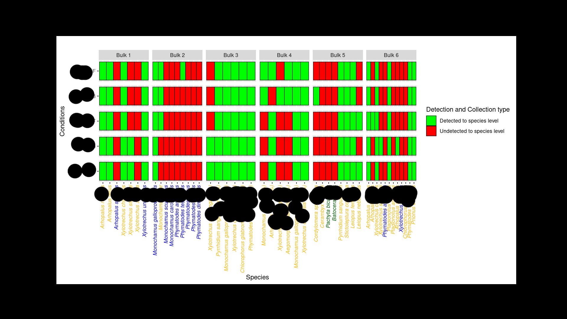
| library(ggplot2)
library(ggtext)
test_data <- read.csv("/home/veillat/Bureau/heatmap.csv")
test_data$Species <- factor(test_data$Species, levels = unique(test_data$Species))
test_data$Conditions <- factor(test_data$Conditions, levels = unique(test_data$Conditions))
# Définition des couleurs en fonction de la colonne "Conservation"
color_mapping <- c("wet" = "blue", "dry" = "darkgoldenrod1", "Hand collected" = "darkgreen")
# Ajouter une colonne avec les étiquettes colorées pour chaque espèce
test_data$Species_Label <- paste0("<i><span style='color:", color_mapping[test_data$Conservation], "'>", test_data$Species, "</span></i>")
# Réorganiser l'ordre des labels de l'axe X
test_data$Species_Label <- factor(test_data$Species_Label, levels = unique(test_data$Species_Label))
# Création du graphique
ggplot(test_data, aes(x = Species_Label, y = Conditions, fill = Detection)) +
geom_raster() +
geom_tile(color = "black", size = 0.3) +
scale_fill_manual(values = c("green", "red")) +
theme(axis.text.x = element_text(angle = 90, vjust = 0.5, hjust = 1, face = "italic"),
strip.text.y = element_blank()) +
ggtitle("") +
facet_grid(rows = vars(Conditions), cols = vars(Bulk), scales = "free", space = "free_y") +
theme(axis.text.x = element_markdown()) +
guides(x = guide_axis(n.dodge = 1)) +
xlab("Species")+
labs(fill = "Detection and Collection type") |


 Répondre avec citation
Partager