Discussion :

[Flo_Phx]

Bonsoir à tous,

je sollicite votre aide pour afficher une abaque dans laquelle il y a deux axes des abscisses (Vitesse conventionnelle et Mach) et un axe unique d'ordonnées (Altitude).

La fonction est de la forme Z = f(X, Y), où j'ai calculé des isomach et des isovitesses. Je souhaiterais que mes axes des abscisses afin, que, par exemple lorsqu'on est à Zp = 0, le point (Vc = 550) soit correctement positionné avec sa valeur en Mach (0,83).

Or, dans l'état actuel de mon développement, l'usage de matplotlib avec deux axes conduit à avoir deux courbes affichées avec deux axes, sans lien entre eux..

Mon objectif est de pouvoir représenter la courbe suivante:


et voici mon code en l'état actuel des choses:

Code :

Sélectionner tout - Visualiser dans une fenêtre à part

1
2
3
4
5
6
7
8
9
10
11
12
13
14
15
16
17
18
19
20
21
22
23
24
25
26
27
28
29
30
31
32
33
34
35
36
37
38
39
40
41
42
43
44
45
46
47
48
49
50
51
52
53
54
55
56
57
58
59
60
61
62
63
64
65
66
67
68
69
70
71
72
73
74
75
76
77
78
79
80
81
82
83
84
85
86
87
88
89
90
91
92
93
94
95
96
97
98
99
100
101
102
103
104
105
106
107
108
109
110
111
112
113
114
115
116
 
# -*- coding: utf-8 -*-
import numpy as np 
from matplotlib import pyplot as plt 
 
##
#
# Modèle ISA
# Valeurs de référence au niveau de la mer 
# MSL = Mean Sea Level
##
MSL_PRESSURE = 101325 # Pression (pa)
MSL_TEMPERATURE_CELSIUS = 15 # Température (°C)
MSL_TEMPERATURE_KELVIN = 288.15 # Température (K)
MSL_rho = 1.225 # kg/m3
 
# Calcul du nombre de mach
# Vc = Vitesse Conventionnelle
COEFF_COMPRESSIBILITE_AIR = 1.4
CSTE_SPECIFIQUE_AIR = 287
 
CSTE_KNOT = 1.852  # 1 noeud = 1.852 km/h
CSTE_FEET = 0.3048 # 1 pied = 0,3048 m
CSTE_ms_kmh = 3.6  # 1 m/s = 3.6 km/h
 
def convertMetertoFeet(meter):
    return meter / CSTE_FEET
 
def convertFeettoMeter(feet):
    return feet * CSTE_FEET
 
#
# 
#
def convertSpeedMsToKmh (speed_ms):
    return speed_ms * CSTE_ms_kmh
 
def convertSpeedKmhToMs (speed_kmh):
    return speed_kmh / CSTE_ms_kmh
 
def convertSpeedKnotToKmh (speed_knot):
    return speed_knot * CSTE_KNOT
 
def convertSpeedKmhToKnot (speed_kmh):
    return speed_kmh / CSTE_KNOT
#
#
#    
def computeStaticPressure(altitude_m):
    return MSL_PRESSURE * (1-(0.0065 * altitude_m)/MSL_TEMPERATURE_KELVIN)**5.255
 
def computeTotalPressure(staticPressure_Pa, machNumber):
    return staticPressure_Pa * (1 + (COEFF_COMPRESSIBILITE_AIR-1) /2 * machNumber**2)**(COEFF_COMPRESSIBILITE_AIR/(COEFF_COMPRESSIBILITE_AIR-1))
 
def computeCalibratedAirSpeed(staticPressure_Pa, totalPressure_Pa):
    exposant = (COEFF_COMPRESSIBILITE_AIR- 1)/COEFF_COMPRESSIBILITE_AIR
    membre_1 = (totalPressure_Pa - staticPressure_Pa)/MSL_PRESSURE
    membre_2 = 2/exposant
    membre_3 = MSL_PRESSURE / MSL_rho
    return np.sqrt((((membre_1 + 1)**exposant - 1)) * membre_2 * membre_3)
 
def computeMachNumber (staticPressure_Pa, Vc_ms):
    step_01 = (COEFF_COMPRESSIBILITE_AIR-1)/(2*COEFF_COMPRESSIBILITE_AIR)
    step_02 = step_01 * (MSL_rho/MSL_PRESSURE) * (Vc_ms **2)
    step_03 = (1 + step_02)**((COEFF_COMPRESSIBILITE_AIR)/(COEFF_COMPRESSIBILITE_AIR - 1)) - 1
    step_04 = (MSL_PRESSURE/staticPressure_Pa) * step_03
    step_05 = (step_04 + 1)**((COEFF_COMPRESSIBILITE_AIR-1)/COEFF_COMPRESSIBILITE_AIR)
    step_06 = 2/(COEFF_COMPRESSIBILITE_AIR-1) * (step_05 - 1)
    return np.sqrt(step_06)
 
 
#conditions initiales des calculs
Zp_Vector_ft = np.arange (0, 36500, 500) # Variation d'altitude par tranche de 500ft
Mach_Vector = np.arange(0, 1, 0.1) # Subsonique : variation par 0,1 point de mach
Vc_Vector_knot = np.arange (0, 560, 50) # Variation de vitesse par tranche de 10 noeuds
 
# Calcul de Ps(Zp)
staticPressure_Vector_Pa = computeStaticPressure(convertFeettoMeter(Zp_Vector_ft))
 
# Calcul de Pt(Ps, M)
totalPressure_Vector_Pa = computeTotalPressure(staticPressure_Vector_Pa[:, None], Mach_Vector)
 
#Calcul de Vc(Ps, Pt)
# staticPressure_Vector_Pa = staticPressure_Vector_Pa[:, None] * np.ones(10)
 
Vc_array = computeCalibratedAirSpeed(staticPressure_Vector_Pa[:, None] * np.ones(10), totalPressure_Vector_Pa)
Vc_array = convertSpeedMsToKmh(Vc_array)
Vc_array = convertSpeedKmhToKnot(Vc_array)
Vc_array = np.around(Vc_array)
 
#Calcul du Mach(Ps, Vc)
Mach_array = computeMachNumber(staticPressure_Vector_Pa[:, None] * np.ones(12), convertSpeedKnotToKmh(convertSpeedKmhToMs(Vc_Vector_knot)))
Mach_array = np.around(Mach_array, 2)
 
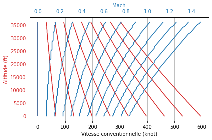
plt.title("Abaque Chevalier") 
plt.xlabel("Vitesse conventionnelle (knot)") 
plt.ylabel("Altitude (ft)") 
plt.grid(True)
 
fig, ax1 = plt.subplots()
 
color = 'tab:red'
ax1.set_xlabel('Vitesse conventionnelle (knot)')
ax1.set_ylabel('Altitude (ft)', color=color)
ax1.plot(Vc_array, Zp_Vector_ft, color=color)
ax1.grid(True)
ax1.tick_params(axis='y', labelcolor=color)
 
ax2 = ax1.twiny()  # instantiate a second axes that shares the same x-axis
 
color = 'tab:blue'
ax2.set_xlabel('Mach', color=color)  # we already handled the x-label with ax1
ax2.plot(Mach_array, Zp_Vector_ft, color=color)
ax2.tick_params(axis='x', labelcolor=color)
fig.tight_layout()  # otherwise the right y-label is slightly clipped
plt.show()

En vous remerciant d'avance de toutes vos idées!!

[lg_53]

Salut

2 possibilités :
- C'est à vous de faire le lien. Puisqu'il y a une constante de proportionnalité entre la quantité de mach et la vitesse, vos isomach vous pouvez les exprimer comme des isovitesses. Et puis après reste a à placer les légendes comme il faut sur l'axe des mach via ce coefficient de proportionalité.
Des exemples ici
https://matplotlib.org/3.1.0/gallery...dary_axis.html

- Renverser le graphe de 90°. Ca vous donne un seul axe x, et 2 axes y. Et pour ça il y a une fonction aussi :
https://matplotlib.org/gallery/subpl...-two-scales-py

PS: Vous auriez pu présenter un code un peu plus synthétique, étant donné que votre problème n'est qu'un souci d'affichage... Donc toute la physique qu'il y a autour elle est certes intéressante, mais dans ce cas précis c'est juste une pollution pour illustrer votre besoin avec matplotlib.

[Flo_Phx]

Bonsoir,

merci de la réponse, je vais regarder comment exploiter au mieux les exemples.

P.S : désolé pour la longueur du code, je voulais qu'il soit exploitable pour toute personne qui répondrait!