1
2
3
4
5
6
7
8
9
10
11
12
13
14
15
16
17
18
19
20
21
22
23
24
25
26
27
28
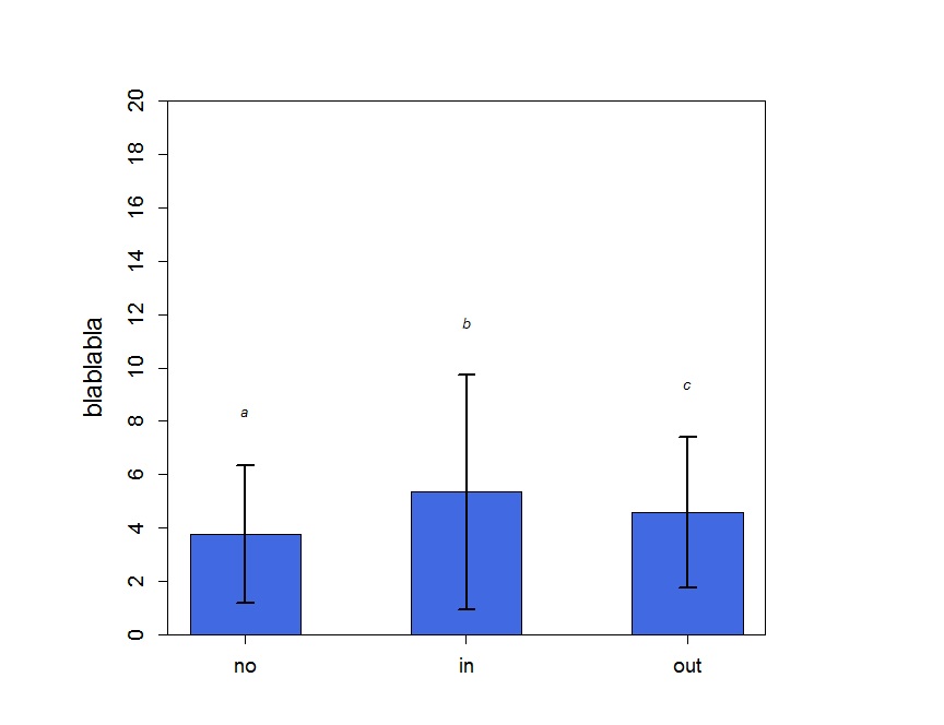
| #troisieme graph histogramme avec sd
x11()
mean<-c(mean(no), mean(in.), mean(out))
graph<-barplot(mean, axes=F, col="royalblue", border="black",
ylim = c(0,20), ylab="blablabla", cex.lab=1.5,
space=1)
# Label axis
axis(1, labels=c("no", "in", "out"), at = graph, cex.axis=1.2)
axis(2, at = seq(min(0), max(20), 2), cex.axis=1.2)
box()
# ajouter les sd
std<-(c(sd(no), sd(in.), sd(out)))
# Plot the vertical lines of the error bars at the midpoints
segments(graph, mean-std, graph,mean+std,lwd=2)
# Now plot the horizontal bounds for the error bars
# 1. The lower bar
segments(graph-0.08, mean-std, graph+0.08, mean-std, lwd=2)
# 2. The upper bar
segments(graph-0.08, mean+std,graph+0.08, mean+std, lwd=2)
# ajouter les stats
text(graph, (mean+std)+2, c("a", "b", "c"), font=3, cex=0.8) |


 Répondre avec citation


Partager