Discussion :

[khoeds]

Bonjour,

Je cherche a faire un spectrogramme (ou sonagramme) d'un fichier wav. J'ai débuté par la version "numpy" définie ci-dessous. Cela m'a permis de comprendre le fonctionnement, mais le temps d’exécution est trop long. Je me suis donc tourné vers des fonction plus optimisées, à savoir "specgram" de "matplotlib.pyplot" et "spectrogram" de "scipy.signal". Je précise que je suis débutant en python, donc excusez-moi d'avance d'erreur "bête" que je pourrait commettre. J'ai réaliser un bout de code pour les comparer :

Code :

Sélectionner tout - Visualiser dans une fenêtre à part

1
2
3
4
5
6
7
8
9
10
11
12
13
14
15
16
17
18
19
20
21
22
23
24
25
26
27
28
29
30
31
32
33
34
35
36
37
38
39
40
41
42
43
44
45
46
47
48
49
50
51
52
53
54
55
56
57
58
59
60
61
62
63
64
65
66
67
68
69
70
71
72
73
74
75
76
77
78
79
80
81
82
83
84
85
86
87
88
89
90
91
92
93
94
95
96
97
98
99
100
101
102
103
104
105
# Import des bibliothèques
 
import matplotlib.pyplot as plot
import numpy as np
from scipy.io import wavfile
from scipy import signal
import time
 
def sonagram_matplotlib(Signal,Fe,L,Chvt,Pas):
    tps=time.time()
    for n in range(0,Chvt-3*Pas,Pas):
        Signal1=Signal[n:]
        spectrum,freqs,t,im = plot.specgram(Signal1,cmap=cmap, Fs=Fe,NFFT=L, noverlap=Chvt, scale='dB')
        t=t+n/Fe
        if n==0:
            Sona_Dict=dict(zip(t,20*np.log10(abs(np.transpose(spectrum)))))
        else:
            Sona_Dict.update(dict(zip(t,20*np.log10(abs(np.transpose(spectrum))))))
 
    t_r=sorted(Sona_Dict)
    Sona=[Sona_Dict[n] for n in t_r]
    Sona=np.transpose(Sona)
    print(time.time()-tps)
    return Sona,freqs,t_r
 
def sonagram_scipy(Signal,Fe,L,Chvt,Pas):
    tps=time.time()
    for n in range(0,Chvt-3*Pas,Pas):
        Signal1=Signal[n:]
        freqs,t,spectrum=signal.spectrogram(Signal1, Fe,noverlap=Chvt, nperseg=L,window='hanning')
        t=t+n/Fe
        if n==0:
            Sona_Dict=dict(zip(t,20*np.log10(abs(np.transpose(spectrum)))))
        else:
            Sona_Dict.update(dict(zip(t,20*np.log10(abs(np.transpose(spectrum))))))
 
    t_r=sorted(Sona_Dict)
    Sona=[Sona_Dict[n] for n in t_r]
    Sona=np.transpose(Sona)
    print(time.time()-tps)
    return Sona,freqs,t_r
 
def sonagram_numpy(Signal,Fe,L,Chvt,Pas):
    tps=time.time()
 
    Npt=np.size(Signal) #nbr de point du signal
    Fenetre=np.hanning(L) #Fenetrage ou "Windowing" ici hanning
 
    Sona=[]
    t=[]
    for n in range(Chvt+1,Npt-L-1,Pas):
        SF=Signal1[n:n+L]*Fenetre #Signal "fenetré"
        SFfft=np.fft.fft(SF,L)
        SFfft_reduit=[20*np.log10(np.abs(SFfft[n])) for n in range(0,int(np.size(SFfft)/2))]
        Sona.append(SFfft_reduit)
        t.append((n+L/2)/Fe)
 
    freqs=np.fft.fftfreq(L,1/Fe)
    freq=[x for x in freqs if x>=0]
    Sona= np.transpose(Sona)    
    print(time.time()-tps)
    return Sona,freq,t
 
#On récupère le signal du fichier wave
Fe1, Signal1 = wavfile.read('cha_rom_aca.wav')
 
L=4096 #Longueur de la section d'analyse en ms (125ms)
Chvt=int(L/2) #Chevauchement ou "overlapping"
pas=int(0.001*Fe1)#nbr de point corresponant à 1ms
cmap = plot.cm.get_cmap('jet')#couleur du sonagramme
 
#On calcul les spectrogrammes suivant différentes méthodes
Sona_matplotlib,freqs_matplotlib,t_matplotlib = sonagram_matplotlib(Signal1,Fe1,L,Chvt,pas)
Sona_scipy,freqs_scipy,t_scipy = sonagram_scipy(Signal1,Fe1,L,Chvt,pas)
Sona_numpy,freqs_numpy,t_numpy = sonagram_numpy(Signal1,Fe1,L,Chvt,pas)
 
#On trace les résultats
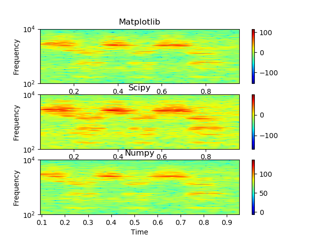
plot.subplot(311) #Resultat matplotlib
plot.pcolormesh(t_matplotlib, freqs_matplotlib, Sona_matplotlib,cmap=cmap)
plot.yscale('log')
plot.ylim(bottom=100, top=10000)
plot.xlabel('Time')
plot.ylabel('Frequency')
plot.title('Matplotlib')
plot.colorbar()
 
plot.subplot(312) #Resultat scipy
plot.pcolormesh(t_scipy, freqs_scipy, Sona_scipy,cmap=cmap)
plot.yscale('log')
plot.ylim(bottom=100, top=10000)
plot.xlabel('Time')
plot.ylabel('Frequency')
plot.title('Scipy')
plot.colorbar()
 
plot.subplot(313) #Resultat numpy
plot.pcolormesh(t_numpy, freqs_numpy, Sona_numpy,cmap=cmap)
plot.yscale('log')
plot.ylim(bottom=100, top=10000)
plot.xlabel('Time')
plot.ylabel('Frequency')
plot.title('Numpy')
plot.colorbar()
 
plot.show()

Le résultat obtenu est le suivant :



Mon problème est le suivant, la forme globale est très ressemblante mais pas identique, c'est une chose. Cependant les valeurs, observables sur les colorbar sont radicalement différentes et je ne comprend pas d'où cela peut venir.

Merci pour l'attention que vous porterez à mon problème ainsi que pour les pistes que vous pourrez m'indiquer.