1
2
3
4
5
6
7
8
9
10
11
12
13
14
15
16
17
18
19
20
21
22
23
24
25
26
27
28
29
30
31
32
33
34
35
36
37
38
39
40
41
42
43
44
45
46
47
48
49
50
51
52
53
54
55
56
57
58
59
60
61
62
63
64
65
66
67
68
69
70
71
72
73
74
75
76
77
78
|
%Time code:
clc;
clear all;
close all;
[y,Fs]=wavread('C:\Users\adee\Desktop\Project Voice Analysis\Part I - my voice\Voice.wav');
T = 1/Fs;
n=length(y);
t=linspace(0,length(y)/Fs,length(y));
figure
plot(t, y, 'g')
%Delete the silence at the beginning:
y = y(:,1);% On travaille en mono
% Calcul de l'énergie (approximation)
S = abs(y);
m = min(S(:));
S = S - m;
M = max(S(:));
S = S/M;
e = S.^2;
% Affichage de e
subplot(312)
figure
plot(e, 'r')
title('~Energie~');
% Seuillage de e
seuil = max(e)*0.2;
e = e>seuil;
% Affichage du seuil
hold on
plot([0 numel(e)],[seuil seuil],'m-')
% Détection des "silences"
index =find(e>seuil);
audiowrite('VoiceSansSilence.wav',y(index(1):index(end)),Fs)
figure
NewY=y(index(1):index(end));
plot(t(index(1):index(end)),NewY)
%FFT code:
NFFT = 2^nextpow2(length(NewY)); % Next power of 2 from length of y
Y = fft(NewY,NFFT)/length(NewY);
f = Fs/2*linspace(0,1,NFFT/2+1);
FFT_signal= Y(1:NFFT/2+1);
% Plot single-sided amplitude spectrum.
figure
plot(f,2*abs(FFT_signal))
title('Spectrum of y(t)')
xlabel('Frequency (Hz)')
ylabel('|Y(f)|')
%Zoom on FFT
figure
idx_3=find(f>0.3e4,1);
plot(f(1:idx_3),abs(FFT_signal(1:idx_3)));
title('Spectrum of y(t) zoomed')
xlabel('Frequency (Hz)')
ylabel('|Y(f)|')
%Parts of the signal
NFFT = 2^nextpow2(length(NewY));
Y=fft(NewY(t>=2 & t<=3),NFFT);
f=-Fs/2:Fs/NFFT:Fs/2-Fs/NFFT; %Making the frequency vector
figure
plot(f,abs(Y));
title('Spectrum of signal(t)');
xlabel('Frequency (Hz)');
ylabel('|signal(f)|'); |


 Répondre avec citation


 pour ce me message
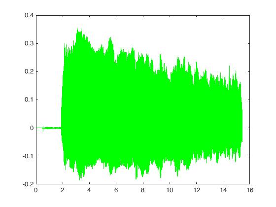

Partager