Discussion :

[simosniper]

Bonjour,
j'ai un problème comme je suis débutant sur MATLAB.
J'ai vraiment besoin de l'aide il me reste peu de temps pour achever mon projet et je me trouve bloqué. Je travaille sur des signaux numériques et
la transformée de Fourier en MATLAB je trouve une difficulté à avoir la solution je vous prie. je vous serai très reconnaissante.



et merci
cordialement

[Invité]

Bonjour,

et je me trouve bloqué.

Par quoi exactement ?
Ne t'attends pas à avoir une solution sur un plateau (Cf règles).

[simosniper]

bonjour,
j'ai fait le 1er exercice

Code :

Sélectionner tout - Visualiser dans une fenêtre à part

1
2
3
4
5
6
7
8
9
10
11
12
13
14
15
16
17
18
19
20
21
22
23
24
25
26
27
28
29
30
31
32
33
34
35
36
37
38
39
40
41
42
43
44
45
46
47
48
49
50
51
52
53
54
55
56
57
58
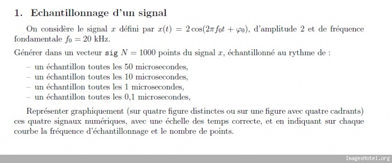
close all
clear all
clc
 
%==========================================================================
% Echantillonnage
 
% Nombre d'echantillons
N=1000;
 
% Frequence fondamentale du signal
fo=20*1000;
 
% Les periodes d'echantillonnage pour [50µs 10µs 1µs 0.1µs]
Te=1e-006*[50,10,1,0.1];
 
% La phase initiale
ro=0;
 
% Frequence echantillonnage =20kHz ==>Te=50µs 
t=0:Te(1):(N-1)*Te(1);
sig=2*cos(2*pi*fo*t+ro);
subplot(2,2,1)
plot(t,sig)
axis([0 N*Te(1) -2.5 2.5])
xlabel('Temps en Seconde')
ylabel('Amplitude')
title('N=1000; Frequence echantillonnage =20kHz')
 
% Frequence echantillonnage =20kHz ==>Te=10µs 
t=0:Te(2):(N-1)*Te(2);
sig=2*cos(2*pi*fo*t+ro);
subplot(2,2,2)
plot(t,sig)
axis([0 N*Te(2) -2.5 2.5])
xlabel('Temps en Seconde')
ylabel('Amplitude')
title('N=1000; Frequence echantillonnage =100kHz')
 
% Frequence echantillonnage =20kHz ==>Te=1µs 
t=0:Te(3):(N-1)*Te(3);
sig=2*cos(2*pi*fo*t+ro);
subplot(2,2,3)
plot(t,sig)
axis([0 N*Te(3) -2.5 2.5])
xlabel('Temps en Seconde')
ylabel('Amplitude')
title('N=1000; Frequence echantillonnage =1MHz')
 
% Frequence echantillonnage =20kHz ==>Te=0.1µs 
t=0:Te(4):(N-1)*Te(4);
sig=2*cos(2*pi*fo*t+ro);
subplot(2,2,4)
plot(t,sig)
axis([0 N*Te(4) -2.5 2.5])
xlabel('Temps en Seconde')
ylabel('Amplitude')
title('N=1000; Frequence echantillonnage =10mHz')

j'ai besoin d'une idée pour le 2eme exercice.

[yass6886]

Bonjour,
As-tu tout simplement regardé l'aide de MATLAB pour la fonction fft?
Tu auras déjà de quoi faire l'exercice 2.