Discussion :

[docmoha]

Bonjour à tous,

Le but de mon travail est d'avoir le signal en rouge dans le graphe ci attaché intitulé "graphe que je cherche à obtenir". Pour mon cas, je n'ai pas réussi à avoir ce signal en rouge. Ci-dessous le programme que j'ai utilisé.

"m" représente la moyenne des deux enveloppes supérieure et inférieure. Mais ce que j'obtiens sont 30 valeurs et le graphe obtenu sont des droites liant ces 30 points. Je cherche un graphe au lieu des droites. J'ai essayé avec une fonction "spline" mais j'ai eu des erreurs, surement une erreur de syntaxe.

Quelqu'un pourra m'aider ? Merci d'avance.

Code :

Sélectionner tout - Visualiser dans une fenêtre à part

1
2
3
4
5
6
7
8
9
10
11
12
13
14
15
16
17
18
19
20
21
22
23
24
25
26
27
28
29
30
31
32
33
34
35
36
37
38
39
40
41
42
43
44
45
46
47
48
49
50
51
52
53
54
55
56
57
58
59
60
61
62
63
64
65
66
67
68
69
70
71
72
73
74
75
76
77
78
79
80
81
82
83
84
85
86
87
88
89
clear all;close all;clc;
fe=1000;
f1=60;f2=25;f3=10;
T=0.5;
N=fe*T;
t=(0:N-1)/(fe);
% déclaration des signaux:
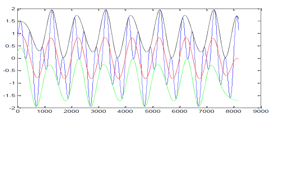
x1=sin(2*pi*f1*t);
x2=sin(2*pi*f2*t);
x3=sin(2*pi*f3*t);
 
x=x1+x2+x3;
 
% Represonttion du signal x(t):
figure
plot(t,x)
grid on
 
%Représentation des signaux x1(t), x2(t), x3(t):
figure(2)
subplot(311)
plot(t,x1)
grid on
subplot(312)
plot(t,x2)
grid on
subplot(313)
plot(t,x3)
grid on
 
 
figure(3)
subplot(311)
plot(t,x)
grid on
 
% 1- calcul des extremums
 
% figure(3)
subplot(312)
plot(t,x,'k')
hold on;
[maxim,imax]= findpeaks(x);
plot(t(imax),maxim,'*r');
% 
hold on;
y=-x;
[minim,imin]=findpeaks(y);
minim=-minim;
plot(t(imin),minim,'*b')
% 
hold off;
grid on
 
%______________________________________________________
 
%2 - Cubic Spline Interpolation
 
subplot(313)
plot(t,x)
 
%######## Enveloppe supérieure #######
 
hold on 
 
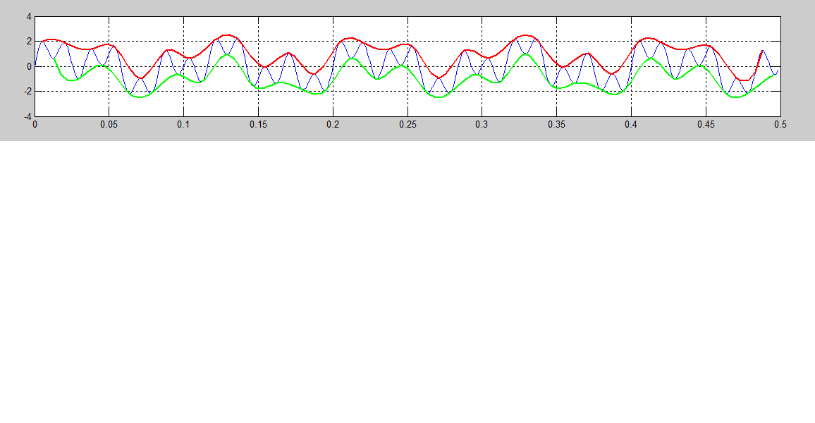
u =spline(t(imax),maxim);
 
fnplt(u,'r');
 
hold on
 
hold off
 
%####### Enveloppe inférieure ########
hold on 
v =spline(t(imin),minim);
fnplt(v,'g');
hold on
hold off
 
 
% 3- Calcul de la moyenne m du signal x 
 
 
hold on
m=(maxim+minim)/2;
plot(m);
hold off
grid on

[Gooby]

Bonjour,

Peux-tu nous montrer les erreurs que tu as rencontré?

[docmoha]

Bonjour,

En fait, le signal moyen que je cherche à obtenir est la demi somme des deux enveloppes u (supérieure) et v (inférieure). C'est à dire :

m(t) = (u(t)+v(t))/2.

En faisant cette somme m = u+v/2 sur MATLAB, j'ai ce message d'erreur :

??? Undefined function or method 'plus' for input arguments of type 'struct'.

Error in ==> Test at 86
m=(u+v)/2;

Merci.

PS: j'ai modifié la ligne 86 du code précédent. m=(u+v)/2 et non pas m=(maxim+minim)/2.

[Gooby]

Tes variables u et v sont des structures, Matlab t'indique qu'il ne peut additionner des structures. Vérifie le contenu de ces variables.

[docmoha]

Les caractéristiques des splines sont :

u =

form: 'pp'
breaks: [1x30 double]
coefs: [29x4 double]
pieces: 29
order: 4
dim: 1

Quelqu'un peut m'aider ??

Merci.

[phryte]

L'accès aux données :

Code :

Sélectionner tout - Visualiser dans une fenêtre à part

1
2
u.coefs
u.breaks

[phryte]

L'accès aux données :

Code :

Sélectionner tout - Visualiser dans une fenêtre à part

1
2
u.coefs
u.breaks

[docmoha]

Quand j'ai mis les deux commandes

Code :

Sélectionner tout - Visualiser dans une fenêtre à part

1
2
u.breaks
v.breaks

c'est une matrice [1x30]. Ce sont des valeurs numériques.

Je bloque toujours sur l'obtention du signal moyen des deux enveloppes supérieure et inférieure.

Merci pour votre aide.

[phryte]

Bonjour.

Pour le signal enveloppe :

Code :

Sélectionner tout - Visualiser dans une fenêtre à part

1
2
3
4
5
6
figure(5)
 [maxim,imax]= findpeaks(x);
 y = spline(t(imax),maxim,t);
 plot(t,x,t,y,'r')
 axis([0 0.5,-4,4])
 grid